

This notebook contains an excerpt from the Python Programming and Numerical Methods - A Guide for Engineers and Scientists, the content is also available at Berkeley Python Numerical Methods.
The copyright of the book belongs to Elsevier. We also have this interactive book online for a better learning experience. The code is released under the MIT license. If you find this content useful, please consider supporting the work on Elsevier or Amazon!
< 8.1 Complexity and Big-O Notation | Contents | 8.3 The Profiler >
Complexity Matters
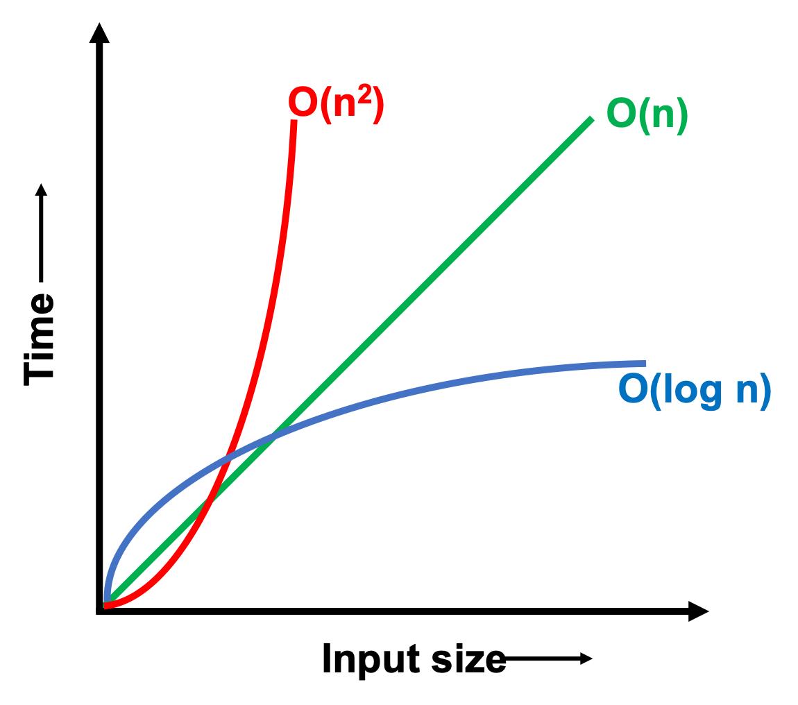
So why does complexity matter? Because different complexity requires different time to complete the task. The following figure is a quick sketch showing you how the time changes with different input size for complexity \(log(n)\), \(n\), \(n^2\).
Let us look at another example. Assume you have an algorithm that runs in exponential time, say \(O(2^n)\), and let \(N\) be the largest problem you can solve with this algorithm using the computational resources you have, denoted by \(R\). \(R\) could be the amount of time you are willing to wait for the function to finish, or \(R\) could be the number of basic operations you watch the computer execute before you get sick of waiting. Using the same algorithm, how large of a problem can you solve given a new computer that is twice as fast?
If we establish \(R = 2^N\), using our old computer, with our new computer we have \(2R\) computational resources; therefore, we want to find \(N^{\prime}\) such that \(2R = 2^{N^{\prime}}\). With some substitution, we can arrive at \(2 \times 2^N = 2^{N^{\prime}}\rightarrow 2^{N+1} = 2^{N^{\prime}}\rightarrow N' = N+1\). So with an exponential time algorithm, doubling your computational resources will allow you to solve a problem one unit larger than you could with your old computer. This is a very small difference. In fact as \(N\) gets large, the relative improvement goes to 0.
With a polynomial time algorithm, you can do much better. This time let’s assume that \(R = N^c\), where \(c\) is some constant larger than one. Then \(2R = {N^{\prime}}^c\), which using similar substitutions as before gets you to \(N^{\prime} = 2^{1/c}N\). So with a polynomial time algorithm with power \(c\), you can solve a problem \(\sqrt[c]{2}\) larger than you could with your old computer. When \(c\) is small, say less than 5, this is a much bigger difference than with the exponential algorithm.
Finally, let us consider a log time algorithm. Let \(R = \log{N}\). Then \(2R = \log{N^{\prime}}\), and again with some substitution we obtain \(N^{\prime} = N^2\). So with the double resources, we can square the size of the problem we can solve!
The moral of the story is that exponential time algorithms do not scale well. That is, as you increase the size of the input, you will soon find that the function takes longer (much longer) than you are willing to wait. For one final example, \(my\_fib\_rec(100)\) would take on the order \(2^{100}\) basic operations to perform. If your computer could do 100 trillion basic operations per second (far faster than the fastest computer on earth), it would take your computer about 400 million years to complete. However, \(my\_fib\_iter(100)\) would take less than 1 nanosecond.
There is both an exponential time algorithm (recursion) and a polynomial time algorithm (iteration) for computing Fibonacci numbers. Given a choice, we would clearly pick the polynomial time algorithm. However, there is a class of problems for which no one has ever discovered a polynomial time algorithm. In other words, there are only exponential time algorithms known for them. These problems are known as NP-Complete, and there is ongoing investigation as to whether polynomial time algorithms exist for these problems. Examples of NP-Complete problems include the Traveling Salesman, Set Cover, and Set Packing problems. Although theoretical in construction, solutions to these problems have numerous applications in logistics and operations research. In fact, some encryption algorithms that keep web and bank applications secure rely on the NP-Complete-ness of breaking them. A further discussion of NP-Complete problems and the theory of complexity is beyond the scope of this book but these problems are very interesting and important to many engineering applications.
import numpy as np
import matplotlib.pyplot as plt

%matplotlib inline
plt.figure(figsize = (12, 8))
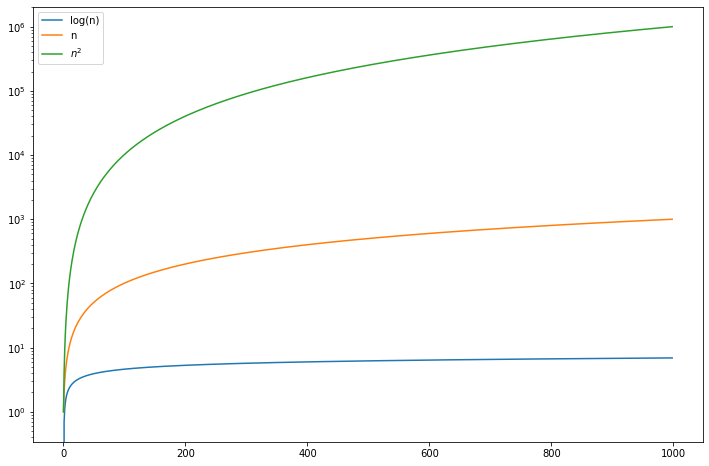
n = np.arange(1, 1e3)
plt.plot(np.log(n), label = 'log(n)')
plt.plot(n, label = 'n')
plt.plot(n**2, label = '$n^2$')
#plt.plot(2**n, label = '$2^n$')
plt.yscale('log')
plt.legend()
plt.show()
< 8.1 Complexity and Big-O Notation | Contents | 8.3 The Profiler >