

This notebook contains an excerpt from the Python Programming and Numerical Methods - A Guide for Engineers and Scientists, the content is also available at Berkeley Python Numerical Methods.
The copyright of the book belongs to Elsevier. We also have this interactive book online for a better learning experience. The code is released under the MIT license. If you find this content useful, please consider supporting the work on Elsevier or Amazon!
< 14.5 Matrix Inversion | Contents | CHAPTER 15. Eigenvalues and Eigenvectors >
Summary
Linear algebra is the foundation of many engineering fields.
Vectors can be considered as points in \({\mathbb{R}}^n\); addition and multiplication are defined on them, although not necessarily the same as for scalars.
A set of vectors is linearly independent if none of the vectors can be written as a linear combination of the others.
Matrices are tables of numbers. They have several important properties including the determinant, rank, and inverse.
A system of linear equations can be represented by the matrix equation \(Ax = y\).
The number of solutions to a system of linear equations is related to the rank(\(A\)) and the rank(\([A,y]\)). It can be zero, one, or infinity.
We can solve the equations using Gauss Elimination, Gauss-Jordan Elimination, LU decomposition and Gauss-Seidel method.
We introduced methods to find matrix inversion.
Problems
Show that matrix multiplication distributes over matrix addition: show \(A(B + C) = AB + AC\) assuming that \(A, B\), and \(C\) are matrices of compatible size.
Write a function my_is_orthogonal(v1,v2, tol), where \(v1\) and \(v2\) are column vectors of the same size and \(tol\) is a scalar value strictly larger than 0. The output should be 1 if the angle between \(v1\) and \(v2\) is within tol of \(\pi/2\); that is, \(|\pi/2 - \theta| < \text{tol}\), and 0 otherwise. You may assume that \(v1\) and \(v2\) are column vectors of the same size, and that \(tol\) is a positive scalar.
# Test cases for problem 2
a = np.array([[1], [0.001]])
b = np.array([[0.001], [1]])
# output: 1
my_is_orthogonal(a,b, 0.01)

# output: 0
my_is_orthogonal(a,b, 0.001)

# output: 0
a = np.array([[1], [0.001]])
b = np.array([[1], [1]])
my_is_orthogonal(a,b, 0.01)

# output: 1
a = np.array([[1], [1]])
b = np.array([[-1], [1]])
my_is_orthogonal(a,b, 1e-10)
Write a function my_is_similar(s1,s2,tol) where \(s1\) and \(s2\) are strings, not necessarily the same size, and \(tol\) is a scalar value strictly larger than 0. From \(s1\) and \(s2\), the function should construct two vectors, \(v1\) and \(v2\), where \(v1[0]\) is the number of ‘a’s in \(s1\), \(v1[1]\) is the number ‘b’s in \(s1\), and so on until \(v1[25]\), which is the number of ‘z’s in \(v1\). The vector \(v2\) should be similarly constructed from \(s2\). The output should be 1 if the absolute value of the angle between \(v1\) and \(v2\) is less than tol; that is, \(|\theta| < \text{tol}\).
Write a function my_make_lin_ind(A), where \({A}\) and \({B}\) are matrices. Let the \({rank(A) = n}\). Then \({B}\) should be a matrix containing the first \(n\) columns of \({A}\) that are all linearly independent. Note that this implies that \({B}\) is full rank.
## Test cases for problem 4

A = np.array([[12,24,0,11,-24,18,15],
              [19,38,0,10,-31,25,9],
              [1,2,0,21,-5,3,20],
              [6,12,0,13,-10,8,5],
              [22,44,0,2,-12,17,23]])

B = my_make_lin_ind(A)

# B = [[12,11,-24,15],
#      [19,10,-31,9],
#      [1,21,-5,20],
#      [6,13,-10,5],
#      [22,2,-12,23]]
Cramer’s rule is a method of computing the determinant of a matrix. Consider an \({n} \times {n}\) square matrix \(M\). Let \(M(i,j)\) be the element of \(M\) in the \(i\)-th row and \(j\)-th column of \(M\), and let \(m_{i,j}\) be the minor of \(M\) created by removing the \(i\)-th row and \(j\)-th column from \(M\). Cramer’s rule says that $\( \text{det(M)} = \sum_{i = 1}^{n} (-1)^{i-1} M(1,i) \text{det}(m_{i,j}). \)$
Write a function my_rec_det(M), where the output is \(det(M)\). The function should use Cramer’s rule to compute the determinant, not Numpy’s function.
What is the complexity of my_rec_det in the previous problem? Do you think this is an effective way of determining if a matrix is singular or not?
Let \({p}\) be a vector with length \({L}\) containing the coefficients of a polynomial of order \({L-1}\). For example, the vector \({p = [1,0,2]}\) is a representation of the polynomial \(f(x) = 1 x^2 + 0 x + 2\). Write a function my_poly_der_mat(p), where \({p}\) is the aforementioned vector, and the output \(D\) is the matrix that will return the coefficients of the derivative of \({p}\) when \({p}\) is left multiplied by \({D}\). For example, the derivative of \(f(x)\) is \(f'(x) = 2x\), and therefore, \(d = Dp\) should yield \({d = [2,0]}\). Note this implies that the dimension of \(D\) is \({L-1} \times {L}\). The point of this problem is to show that integrating polynomials is actually a linear transformation.
Use Gauss Elimination to solve the following equations.
Use Gauss-Jordan Elimination to solve the above equations in problem 8.
Get the lower triangular matrix \(L\) and upper triangular matrix \(U\) from the equations in problem 8.
Show that the dot product distributes across vector addition, that is, show that \(u \cdot (v + w) = u \cdot v + u \cdot w\).
Consider the following network consisting of two power supply stations denoted by \(S1\) and \(S2\) and five power recipient nodes denoted by \(N1\) to \(N5\). The nodes are connected by power lines, which are denoted by arrows, and power can flow between nodes along these lines in both directions.
Let \(d_{i}\) be a positive scalar denoting the power demands for node \(i\), and assume that this demand must be met exactly. The capacity of the power supply stations is denoted by \(S\). Power supply stations must run at their capacity. For each arrow, let \(f_{j}\) be the power flow along that arrow. Negative flow implies that power is running in the opposite direction of the arrow.
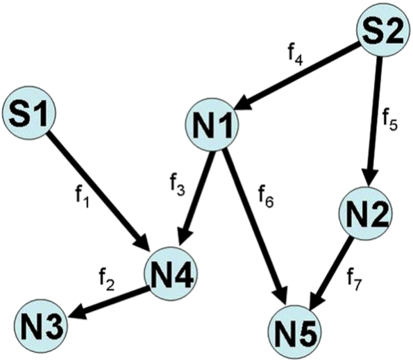
Write a function my_flow_calculator(S, d), where \(S\) is a \(1 \times 2\) vector representing the capacity of each power supply station, and \(d\) is a \(1 \times 5\) row vector representing the demands at each node (i.e., \(d[0]\) is the demand at node 1). The output argument, \(f\), should be a \(1 \times 7\) row vector denoting the flows in the network (i.e., \(f[0] = f_1\) in the diagram). The flows contained in \(f\) should satisfy all constraints of the system, like power generation and demands. Note that there may be more than one solution to the system of equations.
The total flow into a node must equal the total flow out of the node plus the demand; that is, for each node \(i, f_{\text{inflow}} = f_{\text{outflow}} + d_{i}\). You may assume that \(\Sigma{S_j} = \Sigma{d_i}\).
## Test cases for problem 4

s = np.array([[10, 10]])
d = np.array([[4, 4, 4, 4, 4]])

# f = [[10.0, 4.0, -2.0, 4.5, 5.5, 2.5, 1.5]]
f = my_flow_calculator(s, d)

s = np.array([[10, 10]])
d = np.array([[3, 4, 5, 4, 4]])
# f = [[10.0, 5.0, -1.0, 4.5, 5.5, 2.5, 1.5]]
f = my_flow_calculator(s, d)
< 14.5 Matrix Inversion | Contents | CHAPTER 15. Eigenvalues and Eigenvectors >