

This notebook contains an excerpt from the Python Programming and Numerical Methods - A Guide for Engineers and Scientists, the content is also available at Berkeley Python Numerical Methods.
The copyright of the book belongs to Elsevier. We also have this interactive book online for a better learning experience. The code is released under the MIT license. If you find this content useful, please consider supporting the work on Elsevier or Amazon!
< 16.5 Least Square Regression for Nonlinear Functions | Contents | CHAPTER 17. Interpolation >
Summary
Mathematical models are used to understand, predict, and control engineering systems. These models consist of parameters that govern the way the model behaves.
Given a set of experimental data, least squares regression is a method of finding a set of model parameters that fits the data well. That is, it minimizes the squared error between the model, or estimation function, and the data points.
In linear least squares regression, the estimation function must be a linear combination of linearly independent basis functions.
The set of parameters \({\beta}\) can be determined by the least squares equation \({\beta} = (A^T A)^{-1} A^T Y\), where the \(j\)-th column of \(A\) is the \(j\)-th basis function evaluated at each \(X\) data point.
To estimate a nonlinear function, we can transform it into a linear estimation function or directly use least square regression to solve the non-linear function using curve_fit from scipy.
Problems
Repeat the multivariable calculus derivation of the least squares regression formula for an estimation function \(\hat{y}(x) = ax^2 + bx + c\) where \(a, b\), and \(c\) are the parameters.
Write a function my_ls_params(f, x, y), where x and y are arrays of the same size containing experimental data, and f is a list with each element a function object to a basis vector of the estimation function. The output argument, beta, should be an array of the parameters of the least squares regression for x, y, and f.
Write a function my_func_fit (x,y), where x and y are column vectors of the same size containing experimental data, and the function returns alpha and beta are the parameters of the estimation function \(\hat{y}(x) = {\alpha} x^{{\beta}}\).
Given four data points \((x_i, y_i)\) and the parameters for a cubic polynomial \(\hat{y}(x) = ax^3 + bx^2 + cx + d\), what will be the total error associated with the estimation function \(\hat{y}(x)\)? Where can we place another data point (x,y) such that no additional error is incurred for the estimation function?
Write a function my_lin_regression(f, x, y), where f is a list containing function objects to basis functions, and x and y are arrays containing noisy data. Assume that x and y are the same size.
Let an estimation function for the data contained in x and y be defined as \(\hat{y}(x) = {\beta}(1) \cdot f_{1}(x) + {\beta}(2) \cdot f_{2}(x) + \cdots + {\beta}(n) \cdot f_{n}(x)\), where n is the length of f. Your function should compute beta according to the least squares regression formula.
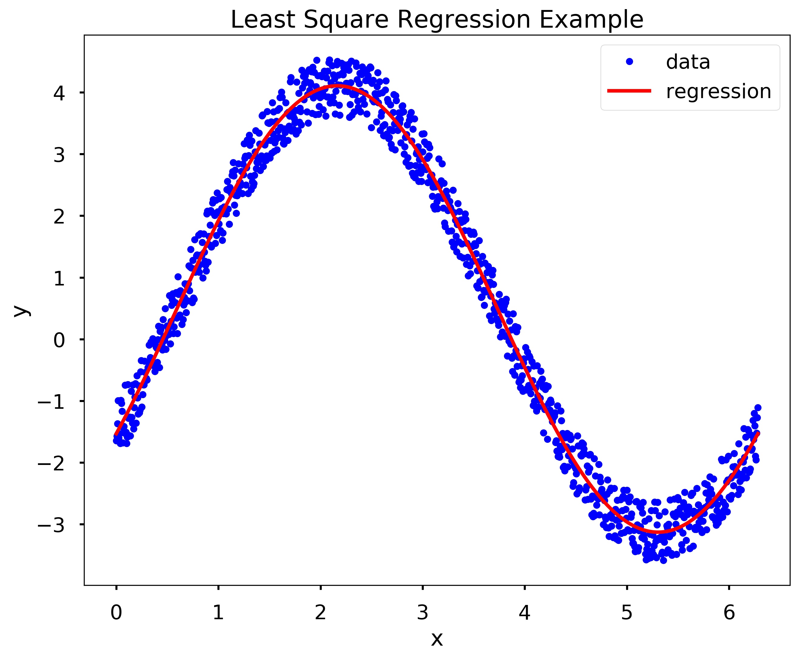
Test Case: Note that your solution may vary by a little bit depending on the random numbers generated.
x = np.linspace(0, 2*np.pi, 1000)
y = 3*np.sin(x) - 2*np.cos(x) + np.random.random(len(x))
f = [np.sin, np.cos]
beta = my_lin_regression(f, x, y)

plt.figure(figsize = (10,8))
plt.plot(x,y,'b.', label = 'data')
plt.plot(x, beta[0]*f[0](x)+beta[1]*f[1](x)+beta[2], 'r', label='regression')
plt.xlabel('x')
plt.ylabel('y')
plt.title('Least Square Regression Example')
plt.legend()
plt.show()
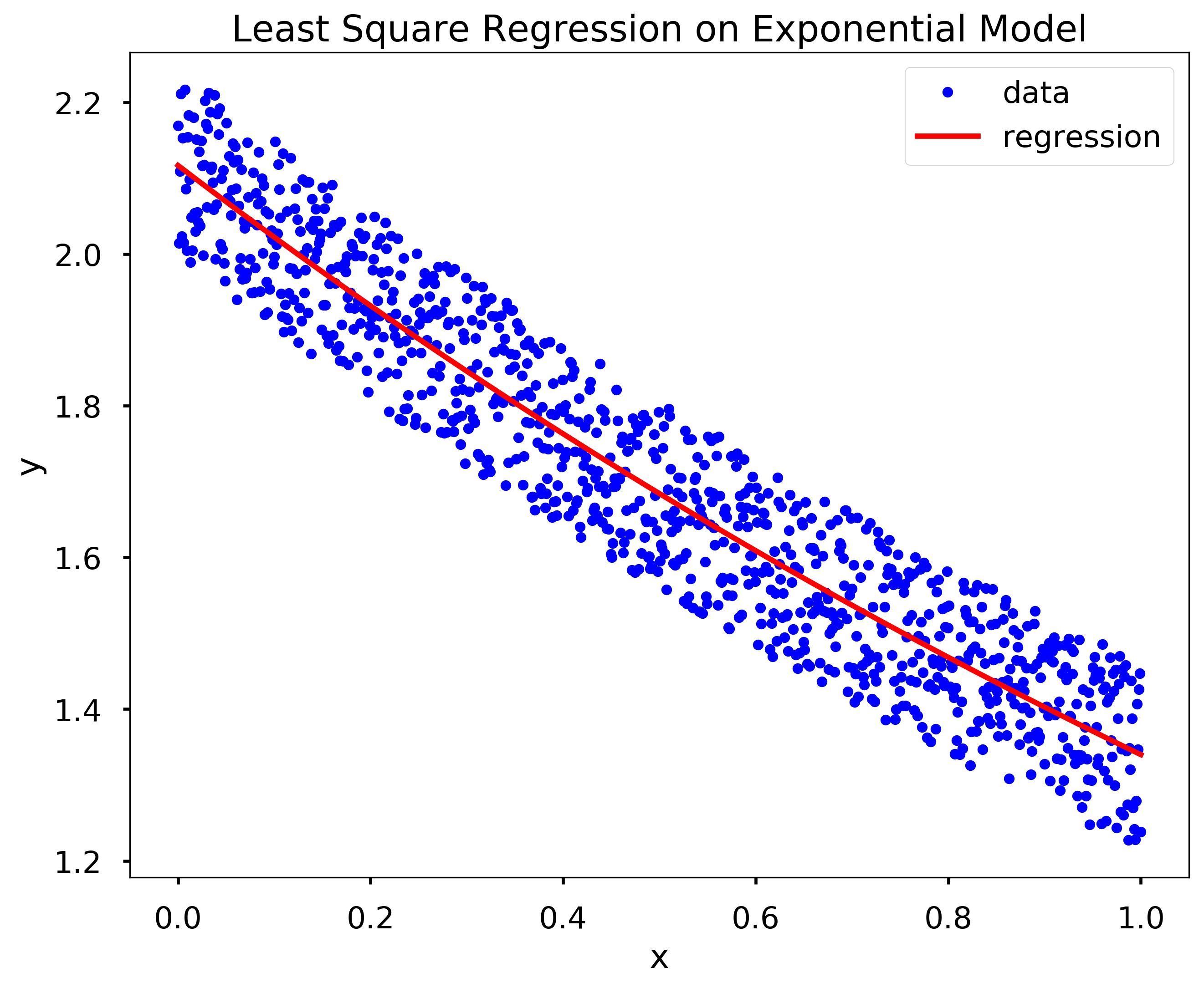
Write a function my_exp_regression (x,y), where x and y are arrays the same size.
Let an estimation function for the data contained in x and y be defined as \(\hat{y}(x) = {\alpha} e^{{\beta} x}\). Your function should compute \({\alpha}\) and \({\beta}\) as the solution to the least squares regression formula.
Test Cases: Note that your solution may vary from the test case slightly depending on the random numbers generated.
x = np.linspace(0, 1, 1000)
y = 2*np.exp(-0.5*x) + 0.25*np.random.random(len(x))

alpha, beta = my_exp_regression(x, y)

plt.figure(figsize = (10,8))
plt.plot(x,y,'b.', label = 'data')
plt.plot(x, alpha*np.exp(beta*x), 'r', label='regression')
plt.xlabel('x')
plt.ylabel('y')
plt.title('Least Square Regression on Exponential Model')
plt.legend()
plt.show()
< 16.5 Least Square Regression for Nonlinear Functions | Contents | CHAPTER 17. Interpolation >