

This notebook contains an excerpt from the Python Programming and Numerical Methods - A Guide for Engineers and Scientists, the content is also available at Berkeley Python Numerical Methods.
The copyright of the book belongs to Elsevier. We also have this interactive book online for a better learning experience. The code is released under the MIT license. If you find this content useful, please consider supporting the work on Elsevier or Amazon!
< 17.1 Interpolation Problem Statement | Contents | 17.3 Cubic Spline Interpolation >
Linear Interpolation
In linear interpolation, the estimated point is assumed to lie on the line joining the nearest points to the left and right. Assume, without loss of generality, that the \(x\)-data points are in ascending order; that is, \(x_i < x_{i+1}\), and let \(x\) be a point such that \(x_i < x < x_{i+1}\). Then the linear interpolation at \(x\) is: $\( \hat{y}(x) = y_i + \frac{(y_{i+1} - y_{i})(x - x_{i})}{(x_{i+1} - x_{i})}.\)$
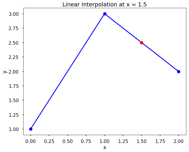
TRY IT! Find the linear interpolation at \(x=1.5\) based on the data x = [0, 1, 2], y = [1, 3, 2]. Verify the result using scipy’s function interp1d.
Since \(1 < x < 2\), we use the second and third data points to compute the linear interpolation. Plugging in the corresponding values gives $\( \hat{y}(x) = y_i + \frac{(y_{i+1} - y_{i})(x - x_{i})}{(x_{i+1} - x_{i})} = 3 + \frac{(2 - 3)(1.5 - 1)}{(2 - 1)} = 2.5 \)$
from scipy.interpolate import interp1d
import matplotlib.pyplot as plt

plt.style.use('seaborn-poster')
x = [0, 1, 2]
y = [1, 3, 2]

f = interp1d(x, y)
y_hat = f(1.5)
print(y_hat)
2.5
plt.figure(figsize = (10,8))
plt.plot(x, y, '-ob')
plt.plot(1.5, y_hat, 'ro')
plt.title('Linear Interpolation at x = 1.5')
plt.xlabel('x')
plt.ylabel('y')
plt.show()
< 17.1 Interpolation Problem Statement | Contents | 17.3 Cubic Spline Interpolation >