

This notebook contains an excerpt from the Python Programming and Numerical Methods - A Guide for Engineers and Scientists, the content is also available at Berkeley Python Numerical Methods.
The copyright of the book belongs to Elsevier. We also have this interactive book online for a better learning experience. The code is released under the MIT license. If you find this content useful, please consider supporting the work on Elsevier or Amazon!
< 17.3 Cubic Spline Interpolation | Contents | 17.5 Newton’s Polynomial Interpolation >
Lagrange Polynomial Interpolation
Rather than finding cubic polynomials between subsequent pairs of data points, Lagrange polynomial interpolation finds a single polynomial that goes through all the data points. This polynomial is referred to as a Lagrange polynomial, \(L(x)\), and as an interpolation function, it should have the property \(L(x_i) = y_i\) for every point in the data set. For computing Lagrange polynomials, it is useful to write them as a linear combination of Lagrange basis polynomials, \(P_i(x)\), where $\( P_i(x) = \prod_{j = 1, j\ne i}^n\frac{x - x_j}{x_i - x_j}, \)$
and $\( L(x) = \sum_{i = 1}^n y_i P_i(x). \)$
Here, \(\prod\) means “the product of” or “multiply out.”
You will notice that by construction, \(P_i(x)\) has the property that \(P_i(x_j) = 1\) when \(i = j\) and \(P_i(x_j) = 0\) when \(i \ne j\). Since \(L(x)\) is a sum of these polynomials, you can observe that \(L(x_i) = y_i\) for every point, exactly as desired.
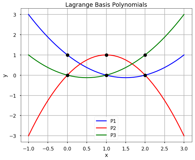
TRY IT! Find the Lagrange basis polynomials for the data set x = [0, 1, 2] and y = [1, 3, 2]. Plot each polynomial and verify the property that \(P_i(x_j) = 1\) when \(i = j\) and \(P_i(x_j) = 0\) when \(i \ne j\).
import numpy as np
import numpy.polynomial.polynomial as poly
import matplotlib.pyplot as plt

plt.style.use('seaborn-poster')
x = [0, 1, 2]
y = [1, 3, 2]
P1_coeff = [1,-1.5,.5]
P2_coeff = [0, 2,-1]
P3_coeff = [0,-.5,.5]

# get the polynomial function
P1 = poly.Polynomial(P1_coeff)
P2 = poly.Polynomial(P2_coeff)
P3 = poly.Polynomial(P3_coeff)

x_new = np.arange(-1.0, 3.1, 0.1)

fig = plt.figure(figsize = (10,8))
plt.plot(x_new, P1(x_new), 'b', label = 'P1')
plt.plot(x_new, P2(x_new), 'r', label = 'P2')
plt.plot(x_new, P3(x_new), 'g', label = 'P3')

plt.plot(x, np.ones(len(x)), 'ko', x, np.zeros(len(x)), 'ko')
plt.title('Lagrange Basis Polynomials')
plt.xlabel('x')
plt.ylabel('y')
plt.grid()
plt.legend()
plt.show()
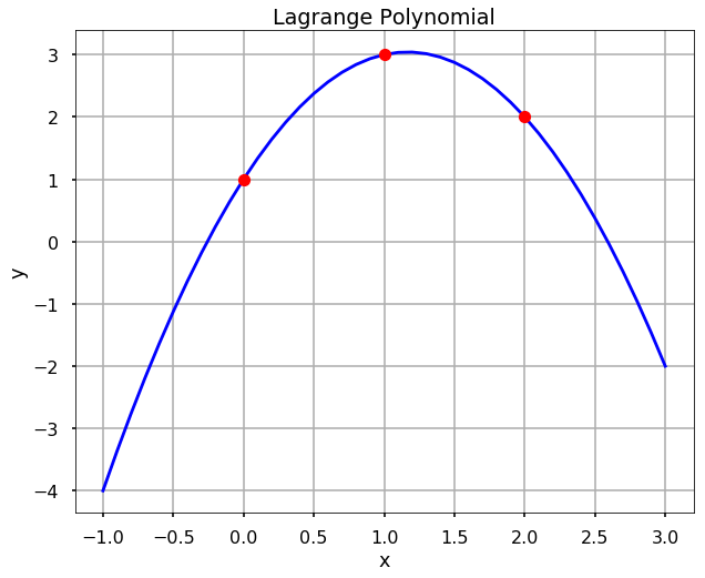
TRY IT! For the previous example, compute and plot the Lagrange polynomial and verify that it goes through each of the data points.
L = P1 + 3*P2 + 2*P3

fig = plt.figure(figsize = (10,8))
plt.plot(x_new, L(x_new), 'b', x, y, 'ro')
plt.title('Lagrange Polynomial')
plt.grid()
plt.xlabel('x')
plt.ylabel('y')
plt.show()

WARNING! Lagrange interpolation polynomials are defined outside the area of interpolation, that is outside of the interval \([x_1,x_n]\), will grow very fast and unbounded outside this region. This is not a desirable feature because in general, this is not the behavior of the underlying data. Thus, a Lagrange interpolation should never be used to interpolate outside this region.
Using lagrange from scipy
Instead of we calculate everything from scratch, in scipy, we can use the lagrange function directly to interpolate the data. Let’s see the above example.
from scipy.interpolate import lagrange
f = lagrange(x, y)
fig = plt.figure(figsize = (10,8))
plt.plot(x_new, f(x_new), 'b', x, y, 'ro')
plt.title('Lagrange Polynomial')
plt.grid()
plt.xlabel('x')
plt.ylabel('y')
plt.show()
< 17.3 Cubic Spline Interpolation | Contents | 17.5 Newton’s Polynomial Interpolation >