

This notebook contains an excerpt from the Python Programming and Numerical Methods - A Guide for Engineers and Scientists, the content is also available at Berkeley Python Numerical Methods.
The copyright of the book belongs to Elsevier. We also have this interactive book online for a better learning experience. The code is released under the MIT license. If you find this content useful, please consider supporting the work on Elsevier or Amazon!
< 18.1 Expressing Functions with Taylor Series | Contents | 18.3 Discussion on Errors >
Approximations with Taylor Series
Clearly, it is not useful to express functions as infinite sums because we cannot even compute them that way. However, it is often useful to approximate functions by using an \(\textbf{\)N^{th}\( order Taylor series approximation}\) of a function, which is a truncation of its Taylor expansion at some \(n = N\). This technique is especially powerful when there is a point around which we have knowledge about a function for all its derivatives. For example, if we take the Taylor expansion of \(e^x\) around \(a = 0\), then \(f^{(n)}(a) = 1\) for all \(n\), we don’t even have to compute the derivatives in the Taylor expansion to approximate \(e^x\)!
TRY IT! Use Python to plot the sin function along with the first, third, fifth, and seventh order Taylor series approximations. Note that this is the zero-th to third in the formula given earlier.
import numpy as np
import matplotlib.pyplot as plt

plt.style.use('seaborn-poster')
x = np.linspace(-np.pi, np.pi, 200)
y = np.zeros(len(x))

labels = ['First Order', 'Third Order', 'Fifth Order', 'Seventh Order']

plt.figure(figsize = (10,8))
for n, label in zip(range(4), labels):
    y = y + ((-1)**n * (x)**(2*n+1)) / np.math.factorial(2*n+1)
    plt.plot(x,y, label = label)

plt.plot(x, np.sin(x), 'k', label = 'Analytic')
plt.grid()
plt.title('Taylor Series Approximations of Various Orders')
plt.xlabel('x')
plt.ylabel('y')
plt.legend()
plt.show()
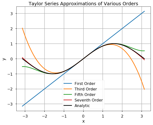
As you can see, the approximation approaches the analytic function quickly, even for \(x\) not near to \(a=0\). Note that in the above code, we also used a new function - zip, which can allow us to loop through two parameters range(4) and labels and use that in our plot.
TRY IT! compute the seventh order Taylor series approximation for \(sin(x)\) around \(a=0\) at \(x=\pi/2\). Compare the value to the correct value, 1.
x = np.pi/2
y = 0

for n in range(4):
    y = y + ((-1)**n * (x)**(2*n+1)) / np.math.factorial(2*n+1)

print(y)
0.9998431013994987
The seventh order Taylor series approximation is very close to the theoretical value of the function even if it is computed far from the point around which the Taylor series was computed (i.e., \(x = \pi/2\) and \(a = 0\)).
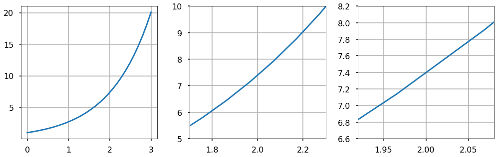
The most common Taylor series approximation is the first order approximation, or linear approximation. Intuitively, for “smooth” functions the linear approximation of the function around a point, \(a\), can be made as good as you want provided you stay sufficiently close to \(a\). In other words, “smooth” functions look more and more like a line the more you zoom into any point. This fact is depicted in the following figure, which we plot successive levels of zoom of a smooth function to illustrate the linear nature of functions locally. Linear approximations are useful tools when analyzing complicated functions locally.
x = np.linspace(0, 3, 30)
y = np.exp(x)

plt.figure(figsize = (14, 4.5))
plt.subplot(1, 3, 1)
plt.plot(x, y)
plt.grid()
plt.subplot(1, 3, 2)
plt.plot(x, y)
plt.grid()
plt.xlim(1.7, 2.3)
plt.ylim(5, 10)
plt.subplot(1, 3, 3)
plt.plot(x, y)
plt.grid()
plt.xlim(1.92, 2.08)
plt.ylim(6.6, 8.2)
plt.tight_layout()
plt.show()
TRY IT! Take the linear approximation for \(e^x\) around the point \(a = 0\). Use the linear approximation for \(e^x\) to approximate the value of \(e^1\) and \(e^{0.01}\). Use Numpy’s function exp to compute exp(1) and exp(0.01) for comparison.
The linear approximation of \(e^x\) around \(a = 0\) is \(1 + x\).
Numpy’s exp function gives the following:
np.exp(1)
2.718281828459045
np.exp(0.01)
1.010050167084168
The linear approximation of \(e^1\) is 2, which is inaccurate, and the linear approximation of \(e^{0.01}\) is 1.01, which is very good. This example illustrates how the linear approximation becomes close to the functions close to the point around which the approximation is taken.
< CHAPTER 18. Series | Contents | 18.2 Approximations with Taylor Series >