

This notebook contains an excerpt from the Python Programming and Numerical Methods - A Guide for Engineers and Scientists, the content is also available at Berkeley Python Numerical Methods.
The copyright of the book belongs to Elsevier. We also have this interactive book online for a better learning experience. The code is released under the MIT license. If you find this content useful, please consider supporting the work on Elsevier or Amazon!
< 21.3 Trapezoid Rule | Contents | 21.5 Computing Integrals in Python >
Simpson’s Rule
Consider two consecutive subintervals, \([x_{i-1}, x_i]\) and \([x_i, x_{i+1}]\). Simpson’s Rule approximates the area under \(f(x)\) over these two subintervals by fitting a quadratic polynomial through the points \((x_{i-1}, f(x_{i-1})), (x_i, f(x_i))\), and \((x_{i+1}, f(x_{i+1}))\), which is a unique polynomial, and then integrating the quadratic exactly. The following shows this integral approximation for an arbitrary function.
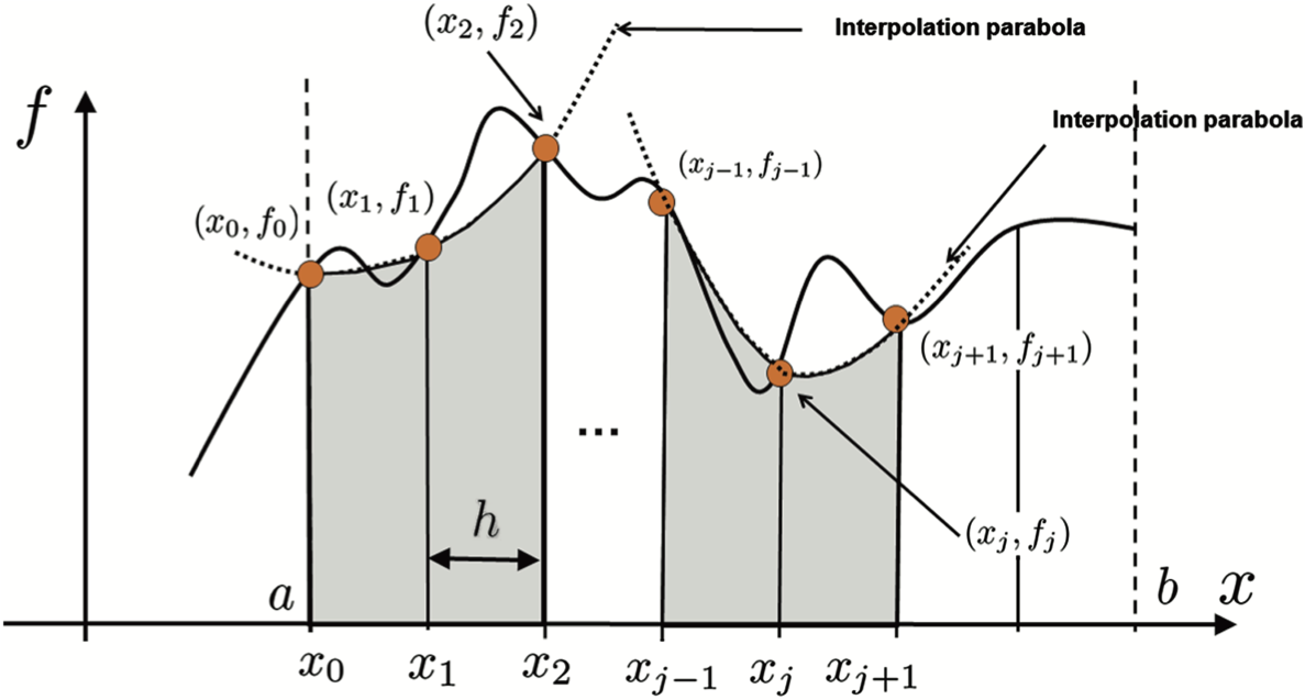
First, we construct the quadratic polynomial approximation of the function over the two subintervals. The easiest way to do this is to use Lagrange polynomials, which was discussed in Chapter 17. By applying the formula for constructing Lagrange polynomials we get the polynomial
and with substitutions for \(h\) results in
You can confirm that the polynomial intersects the desired points. With some algebra and manipulation, the integral of \(P_i(x)\) over the two subintervals is
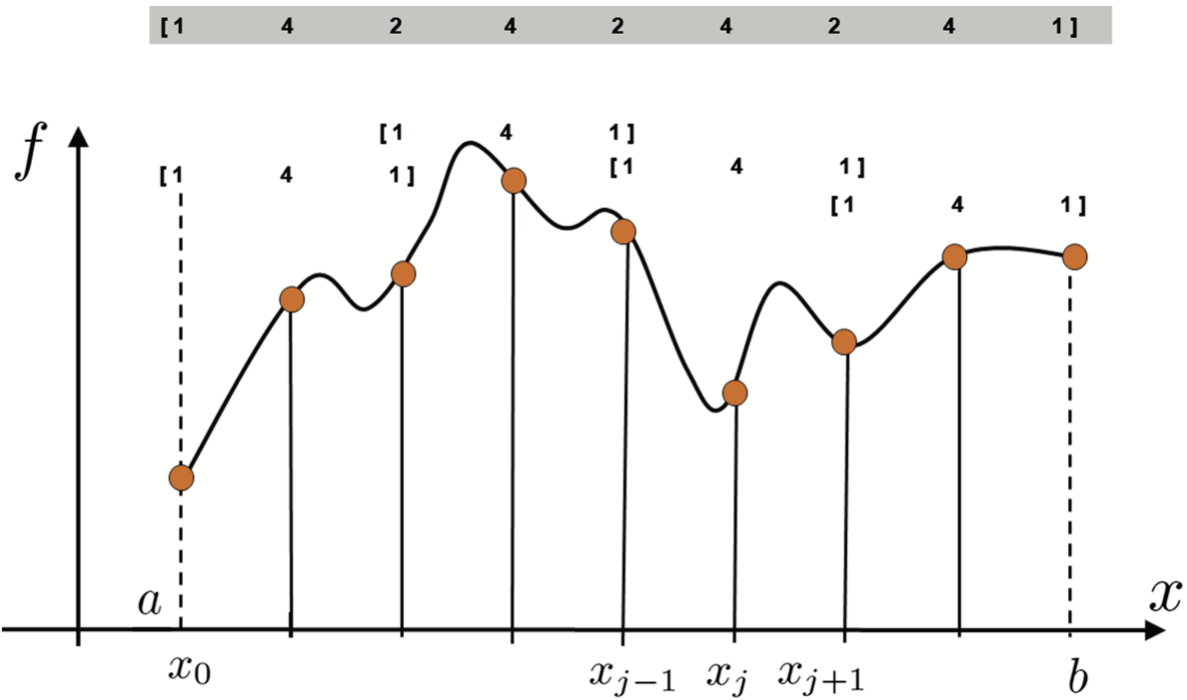
To approximate the integral over \((a, b)\), we must sum the integrals of \(P_i(x)\) over every two subintervals since \(P_i(x)\) spans two subintervals. Substituting \(\frac{h}{3}(f(x_{i-1}) + 4f(x_i) + f(x_{i+1}))\) for the integral of \(P_i(x)\) and regrouping the terms for efficiency leads to the formula
This regrouping is illustrated in the figure below:
WARNING! Note that to use Simpson’s Rule, you must have an even number of intervals and, therefore, an odd number of grid points.
To compute the accuracy of the Simpson’s Rule, we take the Taylor series approximation of \(f(x)\) around \(x_i\), which is
Computing the Taylor series at \(x_{i-1}\) and \(x_{i+1}\) and substituting for \(h\) where appropriate gives the expressions
and
Now consider the expression \(\frac{f(x_{i-1}) + 4f(x_i) + f(x_{i+1})}{6}\). Substituting the Taylor series for the respective numerator values produces the equation
Note that the odd terms cancel out. This implies
By substitution of the Taylor series for \(f(x)\), the integral of \(f(x)\) over two subintervals is then
Again, we distribute the integral and without showing it, we drop the integrals of terms with odd powers because they are zero.
We then carry out the integrations. As will soon be clear, it benefits us to compute the integral of the second term exactly. The resulting equation is
Substituting the expression for \(f(x_i)\) derived earlier, the right-hand side becomes
which can be rearranged to
Canceling and combining the appropriate terms results in the integral expression
Recognizing that \(\frac{h}{3}(f(x_{i-1}) + 4f(x_i) + f(x_{i+1}))\) is exactly the Simpson’s Rule approximation for the integral over this subinterval, this equation implies that Simpson’s Rule is \(O(h^5)\) over a subinterval and \(O(h^4)\) over the whole interval. Because the \(h^3\) terms cancel out exactly, Simpson’s Rule gains another two orders of accuracy!
TRY IT! Use Simpson’s Rule to approximate \(\int_{0}^{\pi} \text{sin} (x)dx\) with 11 evenly spaced grid points over the whole interval. Compare this value to the exact value of 2.
import numpy as np

a = 0
b = np.pi
n = 11
h = (b - a) / (n - 1)
x = np.linspace(a, b, n)
f = np.sin(x)

I_simp = (h/3) * (f[0] + 2*sum(f[:n-2:2]) \
            + 4*sum(f[1:n-1:2]) + f[n-1])
err_simp = 2 - I_simp

print(I_simp)
print(err_simp)
2.0001095173150043
-0.00010951731500430384
< 21.3 Trapezoid Rule | Contents | 21.5 Computing Integrals in Python >