

This notebook contains an excerpt from the Python Programming and Numerical Methods - A Guide for Engineers and Scientists, the content is also available at Berkeley Python Numerical Methods.
The copyright of the book belongs to Elsevier. We also have this interactive book online for a better learning experience. The code is released under the MIT license. If you find this content useful, please consider supporting the work on Elsevier or Amazon!
< CHAPTER 23. Ordinary Differential Equations: Boundary-Value Problems | Contents | 23.2 The Shooting Method >
ODE Boundary Value Problem Statement
In the previous chapter, we talked about ordinary differential equation initial value problems. We can see that in the initial value problems, all the known values are specified at the same value of the independent variable, usually at the lower boundary of the interval, thus this is where the term ‘initial’ comes from. While in this chapter, we will discuss another type of problems - boundary value problems, as the name suggested, the know values are specified at the extremes of the independent variable, therefore, boundaries of the interval.
For example, if we have a simple 2nd order ordinary differential equation,
if the independent variable is over the domain of [0, 20], the initial value problem will have the two conditions on the value 0, that is, we know the value of \(f(0)\) and \(f'(0)\). In contrast, the boundary value problems will specify the values at \(x = 0\) and \(x = 20\). Note that solving a first-order ODE to get a particular solution, we need one constraint, while an \(n\)th-order ODE, we need \(n\) constraints.
The boundary value problem statement for an \(n\)th-order ordinary differential equation is stated as:
To solve this equation on an interval of \(x\in[a, b]\), we need \(n\) known boundary conditions at value \(a\) and \(b\). For the 2nd order case, since we can have the boundary condition either be a value of f(x) or a value of derivative \(f'(x)\), we can have several different cases for the specified values. For example, we can have the boundary condition values specified as:
Two values of \(f(x)\) are given, that is \(f(a)\) and \(f(b)\) are known
Two derivatives of \(f'(x)\) are given, that is \(f'(a)\) and \(f'(b)\) are known
Or mixed conditions from the above two cases are known, that is either \(f(a)\) and \(f'(b)\) are known or \(f'(a)\) and \(f(b)\) are known.
Anyway, to get the particular solution, we need two boundary conditions to get the solution. The second-order ODE boundary value problem is also called Two-Point boundary value problems. The higher order ODE problems need additional boundary conditions, usually the values of higher derivatives of the independent variables. In this chapter, let’s focus on the two-point boundary value problems.
Let’s see an example of the boundary value problem and see how we can solve it in the next few sections.
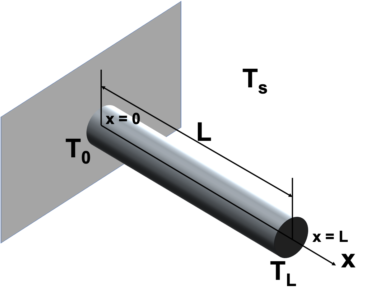
Fins are used in many applications to increase the heat transfer from surfaces. Usually the design of cooling pin fins is encountered in many applications, such as the pin fin used as a heat sink for cooling an object. We can model the temperature distribution in a pin fin as shown in the above figure, where the length of the fin is \(L\), and the start and the end of the fin is \(x=0\) as well as \(x=L\). The temperature at the two ends are \(T_0\) and \(T_L\). \(T_s\) is the temperature of the surrounding environment. If we consider both convection and radiation, the steady-state temperature distribution of the pin fin \(T(x)\) can be modeled with the following equation:
with the boundary conditions: \(T(0) = T_0\) and \(T(L) = T_L\), and \(\alpha_1\) and \(\alpha_2\) are coefficients. This is a second-order ODE with two boundary conditions, therefore, we can solve it to get particular solutions.
The remainder of this chapter covers two methods of numerically approximating the solution to boundary value problems on a numerical grid. We will cover the shooting methods and finite differences methods to solve the boundary value problems ODE.
< CHAPTER 23. Ordinary Differential Equations: Boundary-Value Problems | Contents | 23.2 The Shooting Method >