

This notebook contains an excerpt from the Python Programming and Numerical Methods - A Guide for Engineers and Scientists, the content is also available at Berkeley Python Numerical Methods.
The copyright of the book belongs to Elsevier. We also have this interactive book online for a better learning experience. The code is released under the MIT license. If you find this content useful, please consider supporting the work on Elsevier or Amazon!
< 17.2 Linear Interpolation | Contents | 17.4 Lagrange Polynomial Interpolation >
Cubic Spline Interpolation
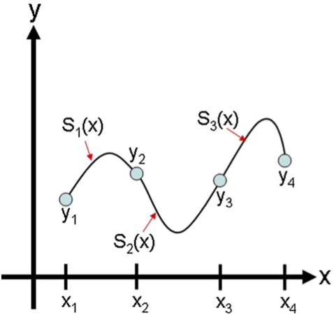
In cubic spline interpolation (as shown in the following figure), the interpolating function is a set of piecewise cubic functions. Specifically, we assume that the points \((x_i, y_i)\) and \((x_{i+1}, y_{i+1})\) are joined by a cubic polynomial \(S_i(x) = a_i x^3 + b_i x^2 + c_i x + d_i\) that is valid for \(x_i \le x \le x_{i+1}\) for \(i = 1,\ldots, n-1\). To find the interpolating function, we must first determine the coefficients \(a_i, b_i, c_i, d_i\) for each of the cubic functions. For \(n\) points, there are \(n-1\) cubic functions to find, and each cubic function requires four coefficients. Therefore we have a total of \(4(n-1)\) unknowns, and so we need \(4(n-1)\) independent equations to find all the coefficients.
First we know that the cubic functions must intersect the data the points on the left and the right:
which gives us \(2(n-1)\) equations. Next, we want each cubic function to join as smoothly with its neighbors as possible, so we constrain the splines to have continuous first and second derivatives at the data points \(i = 2,\ldots,n-1\).
which gives us \(2(n-2)\) equations.
Two more equations are required to compute the coefficients of \(S_i(x)\). These last two constraints are arbitrary, and they can be chosen to fit the circumstances of the interpolation being performed. A common set of final constraints is to assume that the second derivatives are zero at the endpoints. This means that the curve is a “straight line” at the end points. Explicitly,
In Python, we can use scipy’s function CubicSpline to perform cubic spline interpolation. Note that the above constraints are not the same as the ones used by scipy’s CubicSpline as default for performing cubic splines, there are different ways to add the final two constraints in scipy by setting the bc_type argument (see the help for CubicSpline to learn more about this).
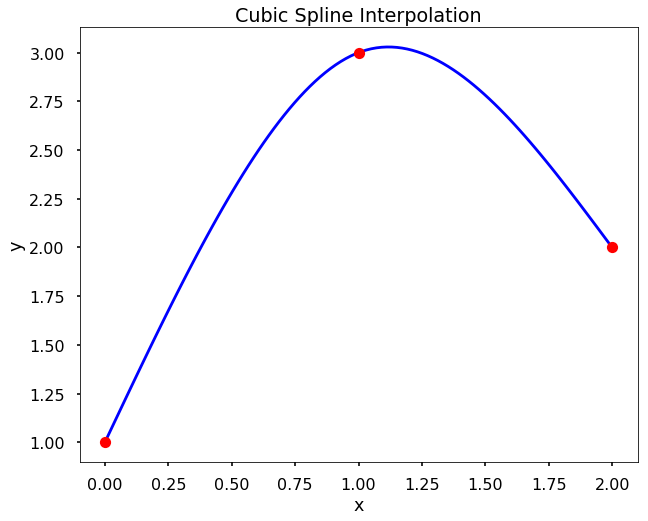
TRY IT! Use CubicSpline to plot the cubic spline interpolation of the data set x = [0, 1, 2] and y = [1, 3, 2] for \(0\le x\le2\).
from scipy.interpolate import CubicSpline
import numpy as np
import matplotlib.pyplot as plt

plt.style.use('seaborn-poster')
x = [0, 1, 2]
y = [1, 3, 2]

# use bc_type = 'natural' adds the constraints as we described above
f = CubicSpline(x, y, bc_type='natural')
x_new = np.linspace(0, 2, 100)
y_new = f(x_new)
plt.figure(figsize = (10,8))
plt.plot(x_new, y_new, 'b')
plt.plot(x, y, 'ro')
plt.title('Cubic Spline Interpolation')
plt.xlabel('x')
plt.ylabel('y')
plt.show()
To determine the coefficients of each cubic function, we write out the constraints explicitly as a system of linear equations with \(4(n-1)\) unknowns. For \(n\) data points, the unknowns are the coefficients \(a_i, b_i, c_i, d_i\) of the cubic spline, \(S_i\) joining the points \(x_i\) and \(x_{i+1}\).
For the constraints \(S_i(x_i) = y_i\) we have: $\( \begin{array}{rrrrr} a_1 x_1^3 + & b_1 x_1^2 + & c_1 x_1 + & d_1 = &y_1,\\ a_2 x_2^3 + & b_2 x_2^2 + & c_2 x_2 + & d_2 = &y_2,\\ \cdots\\ a_{n-1} x_{n-1}^3 + &b_{n-1} x_{n-1}^2 + &c_{n-1} x_{n-1} +& d_{n-1} =& y_{n-1}. \end{array} \)$
For the constraints \(S_i(x_{i+1}) = y_{i+1}\) we have: $\( \begin{array}{rrrrr} a_1 x_2^3 +&b_1 x_2^2 +&c_1 x_2 +&d_1 =& y_2,\\ a_2 x_3^3 +&b_2 x_3^2 +&c_2 x_3 +&d_2 =& y_3,\\ &&\cdots\\ a_{n-1} x_{n}^3 +&b_{n-1} x_{n}^2 +&c_{n-1} x_{n} +&d_{n-1} =& y_{n}. \end{array} \)$
For the constraints \(S^{\prime}_i(x_{i+1}) = S^{\prime}_{i+1}(x_{i+1})\) we have: $\( \begin{array}{rrrrrr} 3a_1 x_2^2 +&2b_1 x_2 +&c_1 - &3a_2 x_2^2 - &2b_2 x_2 - &c_2 =0,\\ 3a_2 x_3^2 +&2b_2 x_3 +&c_2 -& 3a_3 x_3^2 -& 2b_3 x_3 -& c_3 =0,\\ &&&\cdots&&,\\ 3a_{n-2} x_{n-1}^2 +&2b_{n-2} x_{n-1} +&c_{n-2} -& 3a_{n-1} x_{n-1}^2 -& 2b_{n-1} x_{n-1} -& c_{n-1} =0. \end{array} \)$
For the constraints \(S''_i(x_{i+1}) = S''_{i+1}(x_{i+1})\) we have:
Finally for the endpoint constraints \(S''_1(x_1) = 0\) and \(S''_{n-1}(x_n) = 0\), we have: $\( \begin{array}{rr} 6a_1 x_1 +& 2b_1 = 0,\\ 6a_{n-1} x_n +&2b_{n-1} = 0. \end{array} \)$
These equations are linear in the unknown coefficients \(a_i, b_i, c_i\), and \(d_i\). We can put them in matrix form and solve for the coefficients of each spline by left division. Remember that whenever we solve the matrix equation \(Ax = b\) for \(x\), we must make be sure that \(A\) is square and invertible. In the case of finding cubic spline equations, the \(A\) matrix is always square and invertible as long as the \(x_i\) values in the data set are unique.
TRY IT! Find the cubic spline interpolation at x = 1.5 based on the data x = [0, 1, 2], y = [1, 3, 2].
First we create the appropriate system of equations and find the coefficients of the cubic splines by solving the system in matrix form.}
The matrix form of the system of equations is: $\( \left[\begin{array}{llllllll} 0 & 0 & 0 & 1 & 0 & 0 & 0 & 0\\ 0 & 0 & 0 & 0 & 1 & 1 & 1 & 1\\ 1 & 1 & 1 & 1 & 0 & 0 & 0 & 0\\ 0 & 0 & 0 & 0 & 8 & 4 & 2 & 1\\ 3 & 2 & 1 & 0 & -3 & -2 & -1 & 0\\ 6 & 2 & 0 & 0 & -6 & -2 & 0 & 0\\ 0 & 2 & 0 & 0 & 0 & 0 & 0 & 0\\ 0 & 0 & 0 & 0 & 12 & 2 & 0 & 0 \end{array}\right] \left[\begin{array}{c} a_1 \\ b_1 \\ c_1 \\ d_1 \\ a_2 \\ b_2 \\ c_2 \\ d_2 \end{array}\right] = \left[\begin{array}{c} 1 \\ 3 \\ 3 \\ 2 \\ 0 \\ 0 \\ 0 \\ 0 \end{array}\right] \)$
b = np.array([1, 3, 3, 2, 0, 0, 0, 0])
b = b[:, np.newaxis]
A = np.array([[0, 0, 0, 1, 0, 0, 0, 0], [0, 0, 0, 0, 1, 1, 1, 1], [1, 1, 1, 1, 0, 0, 0, 0], \
             [0, 0, 0, 0, 8, 4, 2, 1], [3, 2, 1, 0, -3, -2, -1, 0], [6, 2, 0, 0, -6, -2, 0, 0],\
             [0, 2, 0, 0, 0, 0, 0, 0], [0, 0, 0, 0, 12, 2, 0, 0]])
np.dot(np.linalg.inv(A), b)
array([[-0.75],
       [ 0.  ],
       [ 2.75],
       [ 1.  ],
       [ 0.75],
       [-4.5 ],
       [ 7.25],
       [-0.5 ]])
Therefore, the two cubic polynomials are
So for \(x = 1.5\) we evaluate \(S_2(1.5)\) and get an estimated value of 2.7813.
< 17.2 Linear Interpolation | Contents | 17.4 Lagrange Polynomial Interpolation >