

This notebook contains an excerpt from the Python Programming and Numerical Methods - A Guide for Engineers and Scientists, the content is also available at Berkeley Python Numerical Methods.
The copyright of the book belongs to Elsevier. We also have this interactive book online for a better learning experience. The code is released under the MIT license. If you find this content useful, please consider supporting the work on Elsevier or Amazon!
< 22.2 Reduction of Order | Contents | 22.4 Numerical Error and Instability >
The Euler Method
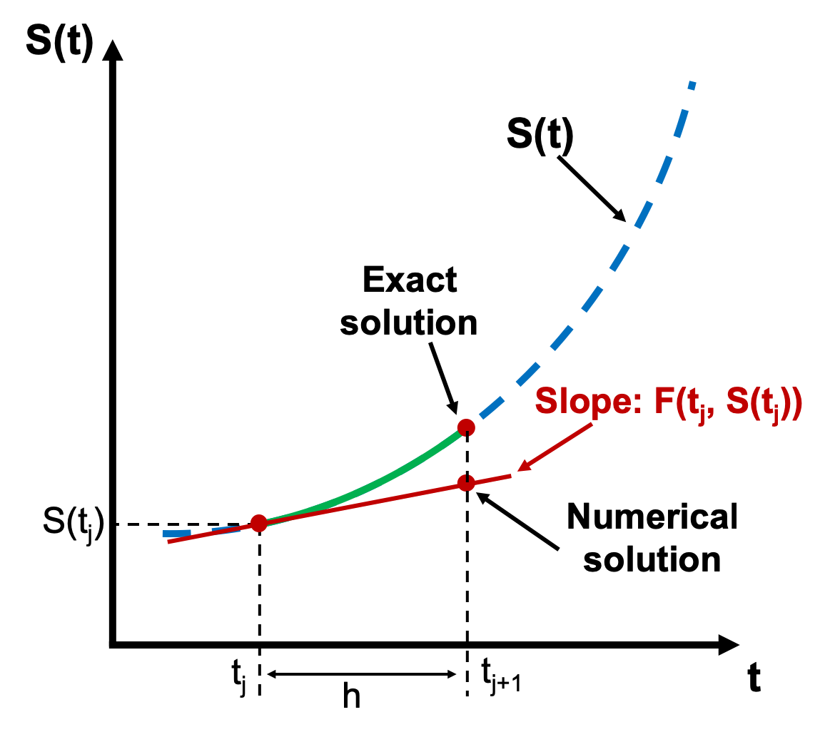
Let dS(t)dt=F(t,S(t)) be an explicitly defined first order ODE. That is, F is a function that returns the derivative, or change, of a state given a time and state value. Also, let t be a numerical grid of the interval [t0,tf] with spacing h. Without loss of generality, we assume that t0=0, and that tf=Nh for some positive integer, N.
The linear approximation of S(t) around tj at tj+1 is
which can also be written
This formula is called the Explicit Euler Formula, and it allows us to compute an approximation for the state at S(tj+1) given the state at S(tj). Starting from a given initial value of S0=S(t0), we can use this formula to integrate the states up to S(tf); these S(t) values are then an approximation for the solution of the differential equation. The Explicit Euler formula is the simplest and most intuitive method for solving initial value problems. At any state (tj,S(tj)) it uses F at that state to “point” toward the next state and then moves in that direction a distance of h. Although there are more sophisticated and accurate methods for solving these problems, they all have the same fundamental structure. As such, we enumerate explicitly the steps for solving an initial value problem using the Explicit Euler formula.
WHAT IS HAPPENING? Assume we are given a function F(t,S(t)) that computes dS(t)dt, a numerical grid, t, of the interval, [t0,tf], and an initial state value S0=S(t0). We can compute S(tj) for every tj in t using the following steps.
Store S0=S(t0) in an array, S.
Compute S(t1)=S0+hF(t0,S0).
Store S1=S(t1) in S.
Compute S(t2)=S1+hF(t1,S1).
Store S2=S(t1) in S.
⋯
Compute S(tf)=Sf−1+hF(tf−1,Sf−1).
Store Sf=S(tf) in S.
S is an approximation of the solution to the initial value problem.
When using a method with this structure, we say the method integrates the solution of the ODE.
TRY IT! The differential equation df(t)dt=e−t with initial condition f0=−1 has the exact solution f(t)=−e−t. Approximate the solution to this initial value problem between 0 and 1 in increments of 0.1 using the Explicity Euler Formula. Plot the difference between the approximated solution and the exact solution.
import numpy as np
import matplotlib.pyplot as plt

plt.style.use('seaborn-poster')
%matplotlib inline

# Define parameters
f = lambda t, s: np.exp(-t) # ODE
h = 0.1 # Step size
t = np.arange(0, 1 + h, h) # Numerical grid
s0 = -1 # Initial Condition

# Explicit Euler Method
s = np.zeros(len(t))
s[0] = s0

for i in range(0, len(t) - 1):
    s[i + 1] = s[i] + h*f(t[i], s[i])

plt.figure(figsize = (12, 8))
plt.plot(t, s, 'bo--', label='Approximate')
plt.plot(t, -np.exp(-t), 'g', label='Exact')
plt.title('Approximate and Exact Solution \
for Simple ODE')
plt.xlabel('t')
plt.ylabel('f(t)')
plt.grid()
plt.legend(loc='lower right')
plt.show()

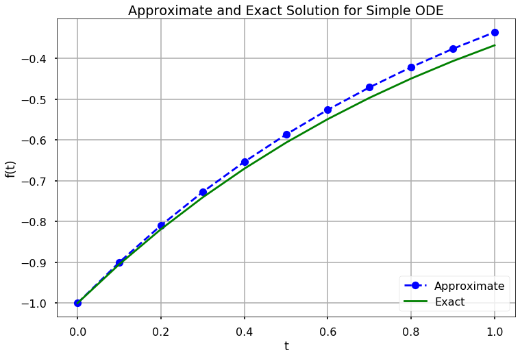
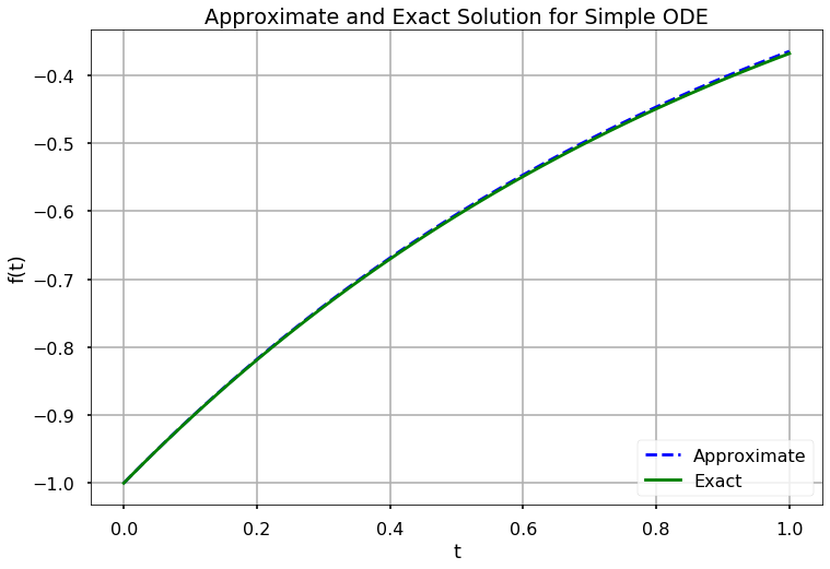
In the above figure, we can see each dot is one approximation based on the previous dot in a linear fashion. From the initial value, we can eventually get an approximation of the solution on the numerical grid. If we repeat the process for h=0.01, we get a better approximation for the solution:
h = 0.01 # Step size
t = np.arange(0, 1 + h, h) # Numerical grid
s0 = -1 # Initial Condition

# Explicit Euler Method
s = np.zeros(len(t))
s[0] = s0

for i in range(0, len(t) - 1):
    s[i + 1] = s[i] + h*f(t[i], s[i])

plt.figure(figsize = (12, 8))
plt.plot(t, s, 'b--', label='Approximate')
plt.plot(t, -np.exp(-t), 'g', label='Exact')
plt.title('Approximate and Exact Solution \
for Simple ODE')
plt.xlabel('t')
plt.ylabel('f(t)')
plt.grid()
plt.legend(loc='lower right')
plt.show()
The Explicit Euler Formula is called “explicit” because it only requires information at tj to compute the state at tj+1. That is, S(tj+1) can be written explicitly in terms of values we have (i.e., tj and S(tj)). The Implicit Euler Formula can be derived by taking the linear approximation of S(t) around tj+1 and computing it at tj:
This formula is peculiar because it requires that we know S(tj+1) to compute S(tj+1)! However, it happens that sometimes we can use this formula to approximate the solution to initial value problems. Before we give details on how to solve these problems using the Implicit Euler Formula, we give another implicit formula called the Trapezoidal Formula, which is the average of the Explicit and Implicit Euler Formulas:
To illustrate how to solve these implicit schemes, consider again the pendulum equation, which has been reduced to first order.
For this equation,
If we plug this expression into the Explicit Euler Formula, we get the following equation:
Similarly, we can plug the same expression into the Implicit Euler to get
and into the Trapezoidal Formula to get
With some rearrangement, these equations become, respectively,
These equations allow us to solve the initial value problem, since at each state, S(tj), we can compute the next state at S(tj+1). In general, this is possible to do when an ODE is linear.
< 22.2 Reduction of Order | Contents | 22.4 Numerical Error and Instability >