

This notebook contains an excerpt from the Python Programming and Numerical Methods - A Guide for Engineers and Scientists, the content is also available at Berkeley Python Numerical Methods.
The copyright of the book belongs to Elsevier. We also have this interactive book online for a better learning experience. The code is released under the MIT license. If you find this content useful, please consider supporting the work on Elsevier or Amazon!
< 22.6 Python ODE Solvers | Contents | 22.8 Summary and Problems >
Advanced Topics
In this section, we will briefly discuss some more advanced topics in IVP ODE. We will not go into the details of them, but if you are interested, we do suggest you check out some great books such as Ordinary Differential Equations by Morris Tenenbaum and Harry Pollard, Numerical Methods for Engineers and Scientists by Amos Gilat and Vish Subramaniam as well as Numerical Methods for Ordinary Differential Equations by J.C. Butcher.
Multistep Methods
So far, most of the methods we discussed are called one-step methods because the approximation for the next point tj+1 is obtained by using information only from S(tj) and tj at the previous point. Although some of the methods, such as RK methods, might use function-evaluation information at points between tj and tj+1, they do not retain the information for direct use in future approximations. The multistep methods attempt to gain efficiency by using two or more previous points to approximate the solution at the next point tj+1. For linear multistep methods, we can use a linear combination of the previous points and derivative values to approximate the next point. The coefficients can be determined using polynomial interpolation we discussed in chapter 17.
There are three families of linear multistep methods are commonly used: Adams–Bashforth methods, Adams–Moulton methods, and the backward differentiation formulas (BDFs).
Stiffness ODE
Stiffness is a difficult and important concept in the numerical solution of ODEs. A stiff ODE equation will make the solution being sought vary slowly, and not stable, i.e. if there are nearby solutions, the solution will change dramatically. This will force us to take small steps to obtain reasonable results. Therefore, stiffness is usually an efficiency issue: if we do not care about computation cost, we would not be concerned about stiffness.
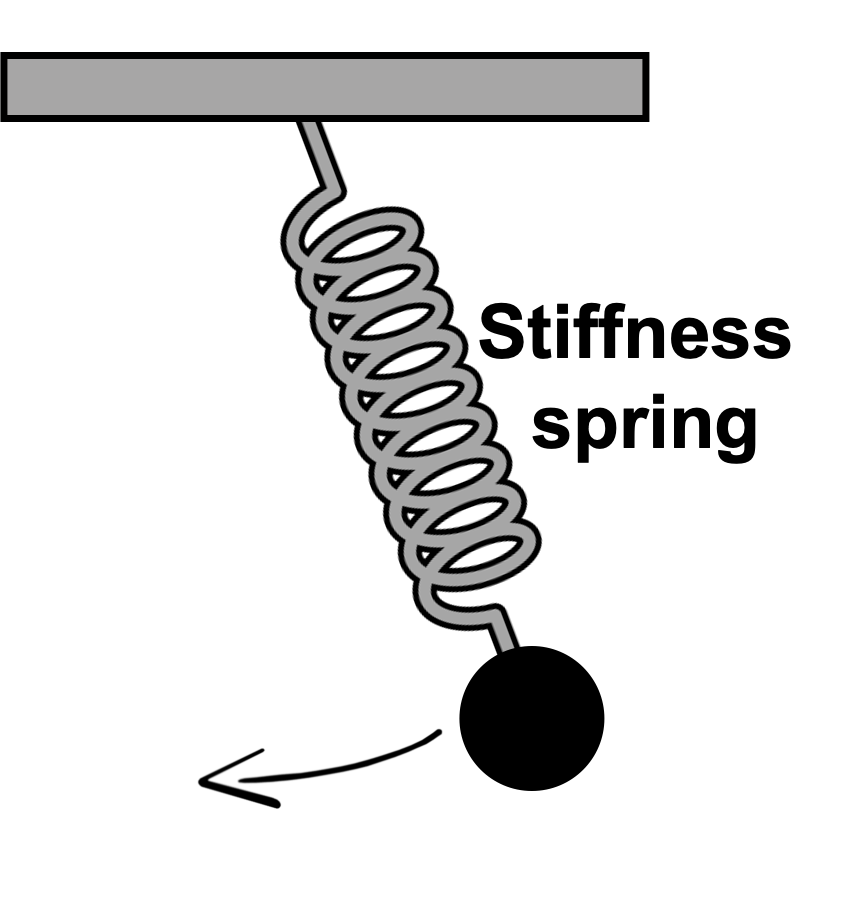
In science and engineering, we often need to model physical phenomena with very different time scales or spatial scales. These applications usually lead to systems of ODEs whose solution include several terms with magnitudes varying with time at a significantly different rate. For example, as the following figure shows a spring mass system, which the mass can swings from left to right as well as oscillates up and down due to the spring. Therefore, we have two different time scales, that is the time scale of the swinging motion as well as the oscillation motion. If the spring is really stiff, thus the oscillation motion time scale will be much smaller than that of the swinging motion. In order to study the system, we have to use a very tiny time step to get a good solution for the oscillation.
Depending on the properties of the ODE and the desired level of accuracy, you might need to use different methods for solve_ivp.There are many methods to choose from for the method argument in solve_ivp; browse through the documentation for additional information. As suggested by the documentation, use the "RK45" or "RK23" method for non-stiff problems and "Radau" or "BDF" for stiff problems. If not sure, first try to run "RK45". Should this solution experience an unusually high number of iterations, diverges, or fails, this problem is likely to be stiff, and you should use "Radau" or "BDF". "LSODA" can also be a good universal choice, but it might be somewhat less convenient to work with as it wraps old Fortran code.
< 22.6 Python ODE Solvers | Contents | 22.8 Summary and Problems >