Trapezoid Rule¶

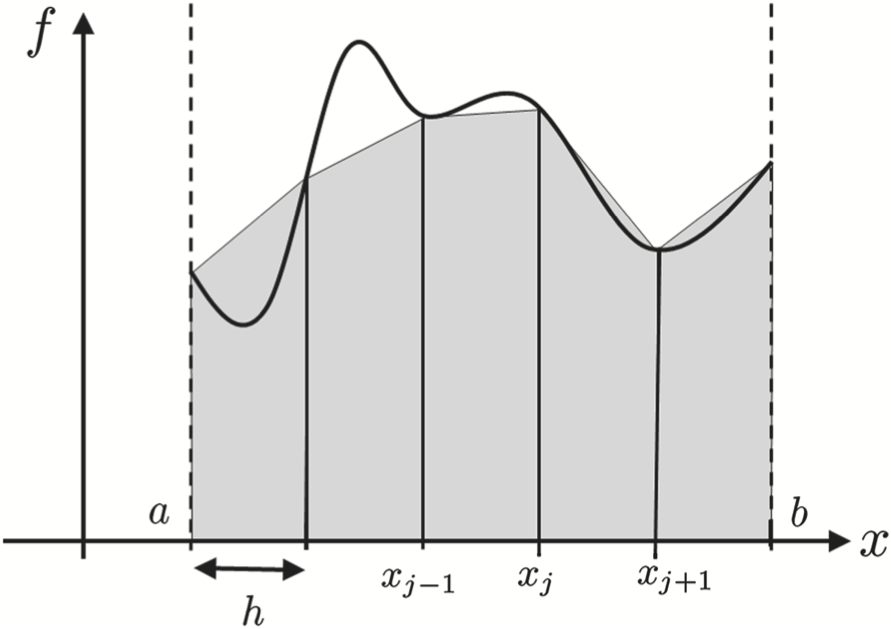
The Trapezoid Rule fits a trapezoid into each subinterval and sums the areas of the trapezoid to approximate the total integral. This approximation for the integral to an arbitrary function is shown in the following figure. For each subinterval, the Trapezoid Rule computes the area of a trapezoid with corners at \((x_i, 0), (x_{i+1}, 0), (x_i, f(x_i))\), and \((x_{i+1}, f(x_{i+1}))\), which is \(h\frac{f(x_i) + f(x_{i+1})}{2}\). Thus, the Trapezoid Rule approximates integrals according to the expression

\[\int_a^b f(x) dx \approx \sum_{i=0}^{n-1} h\frac{f(x_i) + f(x_{i+1})}{2}.\]

TRY IT! You may notice that the Trapezoid Rule “double-counts” most of the terms in the series. To illustrate this fact, consider the expansion of the Trapezoid Rule:

\[\begin{eqnarray*}\sum_{i=0}^{n-1} h\frac{f(x_i) + f(x_{i+1})}{2} &=& \frac{h}{2} \left[(f(x_0) + f(x_1)) + (f(x_1) + f(x_2)) + (f(x_2)\right. \\ &&\left. + f(x_3)) + \cdots + (f(x_{n-1}) + f(x_n))\right].\end{eqnarray*}\]

Computationally, this is many extra additions and calls to \(f(x)\) than is really necessary. We can be more computationally efficient using the following expression.

\[\int_a^b f(x) dx \approx \frac{h}{2} \left(f(x_0) + 2 \left(\sum_{i=1}^{n-1} f(x_i)\right) + f(x_n)\right).\]

To determine the accuracy of the Trapezoid Rule approximation, we first take Taylor series expansion of \(f(x)\) around \(y_i = \frac{x_{i+1} + x_i}{2}\), which is the midpoint between \(x_i\) and \(x_{i+1}\). This Taylor series expansion is

\[f(x) = f(y_i) + f^{\prime}(y_i)(x - y_i) + \frac{f''(y_i)(x - y_i)^2}{2!} + \cdots\]

Computing the Taylor series at \(x_i\) and \(x_{i+1}\) and noting that \(x_i - y_i = -\frac{h}{2}\) and \(x_{i+1} - y_i = \frac{h}{2}\), results in the following expressions:

\[f(x_i) = f(y_i) - \frac{hf^{\prime}(y_i)}{2} + \frac{h^2f''(y_i)}{8} - \cdots\]

and

\[f(x_{i+1}) = f(y_i) + \frac{hf^{\prime}(y_i)}{2} + \frac{h^2f''(y_i)}{8} + \cdots.\]

Taking the average of these two expressions results in the new expression,

\[\frac{f(x_{i+1})+f(x_i)}{2} = f(y_i) + O(h^2).\]

Solving this expression for \(f(y_i)\) yields

\[f(y_i) = \frac{f(x_{i+1})+f(x_i)}{2} + O(h^2).\]

Now returning to the Taylor expansion for \(f(x)\), the integral of \(f(x)\) over a subinterval is

\[\int_{x_i}^{x_{i+1}} f(x) dx = \int_{x_i}^{x_{i+1}} \left(f(y_i) + f^{\prime}(y_i)(x - y_i) + \frac{f''(y_i)(x - y_i)^2}{2!} + \cdots\right) dx.\]

Distributing the integral results in the expression

\[\int_{x_i}^{x_{i+1}} f(x) dx = \int_{x_i}^{x_{i+1}} f(y_i) dx + \int_{x_i}^{x_{i+1}} f^{\prime}(y_i)(x - y_i)dx + \int_{x_i}^{x_{i+1}} \frac{f''(y_i)(x - y_i)^2}{2!} dx + \cdots\]

Now since \(x_i\) and \(x_{i+1}\) are symmetric around \(y_i\), the integrals of the odd powers of \((x - y_i)^p\) disappear and the even powers resolve to a multiple \(h^{p+1}\).

\[\int_{x_i}^{x_{i+1}} f(x) dx = hf(y_i) + O(h^3).\]

Now if we substitute \(f(y_i)\) with the expression derived explicitly in terms of \(f(x_i)\) and \(f(x_{i+1})\), we get

\[\int_{x_i}^{x_{i+1}} f(x) dx = h \left(\frac{f(x_{i+1})+f(x_i)}{2} + O(h^2)\right) + O(h^3), \]

which is equivalent to

\[h \left(\frac{f(x_{i+1})+f(x_i)}{2}\right) + hO(h^2) + O(h^3)\]

and therefore,

\[\int_{x_i}^{x_{i+1}} f(x) dx = h \left(\frac{f(x_{i+1})+f(x_i)}{2}\right) + O(h^3).\]

Since \(\frac{h}{2}(f(x_{i+1}) + f(x_i))\) is the Trapezoid Rule approximation for the integral over the subinterval, it is \(O(h^3)\) for a single subinterval and \(O(h^2)\) over the whole interval.

TRY IT! Use the Trapezoid Rule to approximate \(\int_0^{\pi} \sin(x) dx\) with 11 evenly spaced grid points over the whole interval. Compare this value to the exact value of 2.

import numpy as np

a = 0
b = np.pi
n = 11
h = (b - a) / (n - 1)
x = np.linspace(a, b, n)
f = np.sin(x)

I_trap = (h/2)*(f[0] + \
          2 * sum(f[1:n-1]) + f[n-1])
err_trap = 2 - I_trap

print(I_trap)
print(err_trap)

1.9835235375094546
0.01647646249054535

< 21.2 Riemann’s Integral | Contents | 21.4 Simpson’s Rule >

Python Numerical Methods

Trapezoid Rule¶