

This notebook contains an excerpt from the Python Programming and Numerical Methods - A Guide for Engineers and Scientists, the content is also available at Berkeley Python Numerical Methods.
The copyright of the book belongs to Elsevier. We also have this interactive book online for a better learning experience. The code is released under the MIT license. If you find this content useful, please consider supporting the work on Elsevier or Amazon!
< CHAPTER 22. Ordinary Differential Equations (ODEs): Initial-Value Problems | Contents | 22.2 Reduction of Order >
ODE Initial Value Problem Statement
A differential equation is a relationship between a function, \(f(x)\), its independent variable, \(x\), and any number of its derivatives. An ordinary differential equation or ODE is a differential equation where the independent variable, and therefore also the derivatives, is in one dimension. For the purpose of this book, we assume that an ODE can be written
where \(F\) is an arbitrary function that incorporates one or all of the input arguments, and \(n\) is the order of the differential equation. This equation is referred to as an \(n^{\mathrm{th}}\) order ODE.
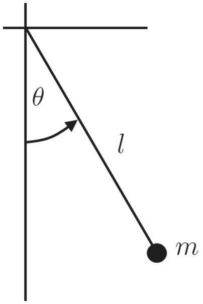
To give an example of an ODE, consider a pendulum of length \(l\) with a mass, \(m\), at its end (see the figure above). The angle the pendulum makes with the vertical axis over time, \(\Theta(t)\), in the presence of vertical gravity, \(g\), can be described by the pendulum equation, which is the ODE
This equation can be derived by summing the forces in the \(x\) and \(y\) direction, and then changing to polar coordinates.
In contrast, a partial differential equation or PDE is a general form differential equation where \(x\) is a vector containing the independent variables \(x_1, x_2, x_3, \ldots, x_m\), and the partial derivatives can be of any order and with respect to any combination of variables. An example of a PDE is the heat equation, which describes the evolution of temperature in space over time:
Here, \(u(t, x, y, z)\) is the temperature at \((x,y,z)\) at time \(t\), and \(\alpha\) is a thermal diffusion constant.
A general solution to a differential equation is a \(g(x)\) that satisfies the differential equation. Although there are usually many solutions to a differential equation, they are still hard to find. For an ODE of order \(n\), a particular solution is a \(p(x)\) that satisfies the differential equation and n explicitly known values of the solution, or its derivatives, at certain points. Generally stated, \(p(x)\) must satisfy the differential equation and \(p^{(j)}(x_i) = p_i\), where \(p^{(j)}\) is the \(j^{\mathrm{th}}\) derivative of \(p\), for \(n\) triplets, \((j, x_i, p_i)\). For the purpose of this text, we refer to the particular solution simply as the solution.
TRY IT! Returning to the pendulum example, if we assume the angles are very small (i.e., \(\sin(\Theta(t)) \approx \Theta(t)\)), then the pendulum equation reduces to
Verify that \(\Theta(t) = \cos\left(\sqrt{\frac{g}{l}}t\right)\) is a general solution to the pendulum equation. If the angle and angular velocities at \(t = 0\) are the known values, \(\Theta_0\) and 0, respectively, verify that \(\Theta(t) = \Theta_0\cos\left(\sqrt{\frac{g}{l}}t\right)\) is a particular solution for these known values.
For the general solution, the derivatives of \(\Theta(t)\) are
and
By plugging the second derivative back into the differential equation on the left side, it is easy to verify that \(\Theta(t)\) satisfies the equation and so is a general solution.
For the particular solution, the \(\Theta_0\) coefficient will carry through the derivatives, and it can be verified that the equation is satisfied. \(\Theta(0) = \Theta_0 \cos(0) = \Theta_0\), and \(0 = -\Theta_0 \sqrt{\frac{g}{l}}\sin(0) = 0\), therefore the particular solution also satisfies the known values.
A pendulum swinging at small angles is a very uninteresting pendulum indeed. Unfortunately, there is no explicit solution for the pendulum equation with large angles that is as simple algebraically. Since this system is much simpler than most practical engineering systems and has no obvious analytic solution, the need for numerical solutions to ODEs is clear.
A common set of known values for an ODE solution is the initial value. For an ODE of order \(n\), the initial value is a known value for the \(0^{\mathrm{th}}\) to \((n-1)^{\mathrm{th}}\) derivatives at \(x = 0, f(0), f^{(1)}(0), f^{(2)}(0),\ldots, f^{(n-1)}(0)\). For a certain class of ordinary differential equations, the initial value is sufficient to find a unique particular solution. Finding a solution to an ODE given an initial value is called the initial value problem. Although the name suggests we will only cover ODEs that evolve in time, initial value problems can also include systems that evolve in other dimensions such as space. Intuitively, the pendulum equation can be solved as an initial value problem because under only the force of gravity, an initial position and velocity should be sufficient to describe the motion of the pendulum for all time afterward.
The remainder of this chapter covers several methods of numerically approximating the solution to initial value problems on a numerical grid. Although initial value problems encompass more than just differential equations in time, we use time as the independent variable. We also use several notations for the derivative of \(f(t): f^{\prime}(t), f^{(1)}(t), \frac{df(t)}{dt}\), and \(\dot{f}\), whichever is most convenient for the context.
< CHAPTER 22. Ordinary Differential Equations (ODEs): Initial-Value Problems | Contents | 22.2 Reduction of Order >