.ipynb .pdf

repository

Contents

This notebook contains an excerpt from the Python Programming and Numerical Methods - A Guide for Engineers and Scientists, the content is also available at Berkeley Python Numerical Methods.

The copyright of the book belongs to Elsevier. We also have this interactive book online for a better learning experience. The code is released under the MIT license. If you find this content useful, please consider supporting the work on Elsevier or Amazon!

< 23.5 Python ODE Solvers | Contents | CHAPTER 24. Fourier Transforms >

Summary

1. Boundary value problems are a specific kind of ODE solving problem with boundary conditions specified at the start and end of the interval.

2. The shooting method can transform the boundary value problems to initial value problems and use the root-finding method to solve it.

3. The finite difference method uses the finite difference scheme to approximate the derivatives and turns the problem into a set of equations to solve.

4. The accuracy and stability of the boundary value problems have both similarity and difference to the initial value problems.

Problems

1. Describe the difference between boundary value problems and the initial value problems in ODE.

2. Try to describe the intuition behind the shooting method and how it links to the initial value problems.

3. What is the finite difference method for boundary value problems? How to solve it?

4. Solve the following boundary value problems with $y(0)=0$ and $y(\pi/2)=1$ $$y''+(1-0.2x)y^2=0$$

5. Solve the following ODE with $y(0)=0$ and $y(\pi)=0$ $$y''+siny+1=0$$

6. Given the ODE with the boundary conditions $y(0) = 0$ and $y(12) =0$, $$y'' + 0.5x^2 - 6x =0$$what's the value of$y’(0)$?

7. Solve the following ODE with boundary conditions $y(1) = 0$, $y''(1)=0$ and $y(2) = 1$ $$y''' + \frac{1}{x}y'' - \frac{1}{x^2}y' - 0.1(y')^3 = 0$$

8. A flexible cable is suspended between two points as shown in the following figure. The density of the cable is uniform. The shape of the cable $y(x)$ is governed by the differential equation: $$\frac{d^2y}{d^2x} = C \sqrt{1 + \Big( \frac{dy}{dx} \Big)^2}$$where$C$is a constant that equal to the ratio fo the weight per unit length of the cable to the magnitude of the horizontal component of tension in the cable at its lowest point. The cable hangs between two points specified by$y(0) = 8$m and$y(10) = 10 $m, and C = 0.039$m^{-1}$. Can you determine and plot the shape of the cable between$x = 0$and$x = 10$?

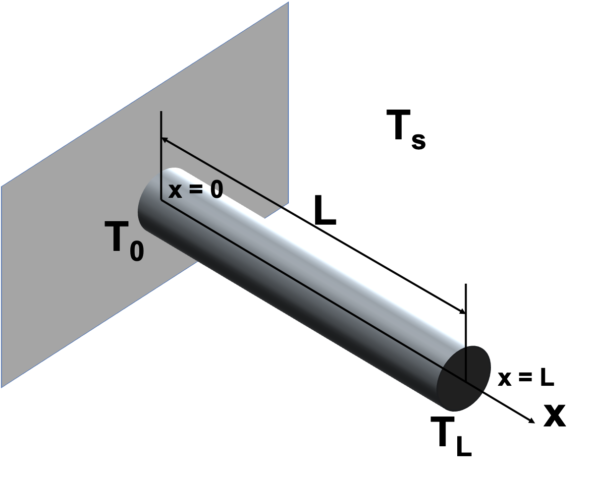
9. Fins are used in many applications to increase the heat transfer from surfaces. Usually the design of cooling pin fins is encountered in many applications, such as the pin fin used as a heat sink for cooling an object. We can model the temperature distribution in a pin fin as shown in the following figure, where the length of the fin is $L$, and the start and the end of the fin is $x=0$ as well as $x=L$. The temperature at the two ends are $T_0$ and $T_L$. $T_s$ is the temperature of the surrounding environment. If we consider both convection and radiation, the steady-state temperature distribution of the pin fin $T(x)$ between $x=0$ and $x=L$ can be modeled with the following equation:

$$\frac{d^2T}{dx^2} - \alpha_1(T - T_s) - \alpha_2(T^4 - T^4) = 0$$

with the boundary conditions: $T(0) = T_0$ and $T(L) = T_L$, and $\alpha_1$ and $\alpha_2$ are coefficients. And they are defined as $\alpha_1 = \frac{h_cP}{kA_c}$ and $\alpha_2 = \frac{\epsilon\sigma_{SB}P}{kA_c}$, where $h_c$ is the convective heat transfer coefficient, $P$ is the perimeter bounding the cross section of the fin, $\epsilon$ is the radiative emissivity of the surface of the fin, $k$ is the thermal conductivity of the fin material, $A_c$ is the cross-sectional area of the fin, and $\sigma_{SB} = 5.67 \times 10^{-8} W/(m^2K^2)$ is the Stefan-Boltzmann constant.

Determine the temperature distribution if $L=0.2$ m, $T(0)=475K$, $T(0.1) = 290 K$, and $T_s = 290 K$. Use the following values for the parameters $h_c = 40 W/m^2/K$, $P=0.015$ m, $\epsilon = 0.4$, $k=240 W/m/K$, and $A_c=1.55 \times 10^{-5} m^2$

1. The simply supported beam carries a uniform load of intensity $q$ as shown in the following figure.

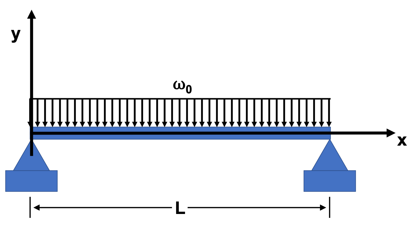
The deflection of the beam, $y$, is governed by the following ODE:

$$EI\frac{d^2y}{dx^2} = \frac{1}{2}\omega_0(Lx-x^2)\Big[ 1 + \Big( \frac{dy}{dx}^2 \Big)\Big]^{\frac{3}{2}}$$

where $EI$ is the flexural rigidity.

If $L=5$ m, and the two boundary conditions are $y(0) = 0$ and $y(L) = 0$, $EI = 1.8 \times 10^7 N-m^2$, and $\omega_0 = 15 \times 10^3 N/m$, determine and plot the deflection of the beam as a function of $x$.

< 23.5 Python ODE Solvers | Contents | CHAPTER 24. Fourier Transforms >

Python ODE Solvers (BVP) Chapter 24. Fourier Transform